Working with large catalogs#
Large astronomical surveys contain a massive volume of data. Billion object, multi-terabyte sized catalogs are challenging to store and manipulate because they demand state-of-the-art hardware. Processing them is expensive, both in terms of runtime and memory consumption, and performing it in a single machine has become impractical. LSDB is a solution that enables scalable algorithm execution. It handles loading, querying, filtering and crossmatching astronomical data (of HiPSCat format) in a distributed environment.
In this tutorial, we will demonstrate how to:
Setup a Dask client for distributed processing
Load an object catalog with a set of desired columns
Select data from regions of the sky
Preview catalog data
[1]:
import lsdb
Installing dependencies#
To load catalogs from the web using the HTTP protocol we’ll need to install aiohttp.
[2]:
!pip install aiohttp --quiet
Creating a Dask client#
Dask is a framework that allows us to take advantage of distributed computing capabilities.
With Dask, the operations defined in a workflow (e.g. this notebook) are added to a task graph which optimizes their order of execution. The operations are not immediately computed, that’s for us to decide. As soon as we trigger the computations, Dask distributes the workload across its multiple workers and tasks are run efficiently in parallel. Usually the later we kick off the computations the better.
Dask creates a client by default, if we do not instantiate one. If we do, we may, among others:
Specify the number of workers and the memory limit for each of them.
Adjust the address for the dashboard to profile the operations while they run (by default it serves on port 8787).
For additional information please refer to https://distributed.dask.org/en/latest/client.html.
[3]:
from dask.distributed import Client

client = Client(n_workers=4, memory_limit="auto")
client
[3]:
Client
Client-d9627a98-0e36-11ef-8575-0242ac110002
| Connection method: Cluster object | Cluster type: distributed.LocalCluster |
| Dashboard: http://127.0.0.1:8787/status |
Cluster Info
LocalCluster
bea35657
| Dashboard: http://127.0.0.1:8787/status | Workers: 4 |
| Total threads: 4 | Total memory: 13.09 GiB |
| Status: running | Using processes: True |
Scheduler Info
Scheduler
Scheduler-04ff79d5-d566-4408-880f-88a864cf1809
| Comm: tcp://127.0.0.1:41983 | Workers: 4 |
| Dashboard: http://127.0.0.1:8787/status | Total threads: 4 |
| Started: Just now | Total memory: 13.09 GiB |
Workers
Worker: 0
| Comm: tcp://127.0.0.1:38765 | Total threads: 1 |
| Dashboard: http://127.0.0.1:44607/status | Memory: 3.27 GiB |
| Nanny: tcp://127.0.0.1:38335 | |
| Local directory: /tmp/dask-scratch-space/worker-318le869 | |
Worker: 1
| Comm: tcp://127.0.0.1:43819 | Total threads: 1 |
| Dashboard: http://127.0.0.1:35935/status | Memory: 3.27 GiB |
| Nanny: tcp://127.0.0.1:41103 | |
| Local directory: /tmp/dask-scratch-space/worker-6vzp5w5m | |
Worker: 2
| Comm: tcp://127.0.0.1:44705 | Total threads: 1 |
| Dashboard: http://127.0.0.1:45357/status | Memory: 3.27 GiB |
| Nanny: tcp://127.0.0.1:34033 | |
| Local directory: /tmp/dask-scratch-space/worker-st1a4rad | |
Worker: 3
| Comm: tcp://127.0.0.1:46153 | Total threads: 1 |
| Dashboard: http://127.0.0.1:34411/status | Memory: 3.27 GiB |
| Nanny: tcp://127.0.0.1:42451 | |
| Local directory: /tmp/dask-scratch-space/worker-3_zxas5f | |
Loading a catalog#
We will load a small 5 degree radius cone from the ZTF DR14 object catalog.
Catalogs represent tabular data and are internally subdivided into partitions based on their positions in the sky. When processing a catalog, each worker is expected to be able to load a single partition at a time into memory for processing. Therefore, when loading a catalog, it’s crucial to specify the subset of columns we need for our science pipeline. Failure to specify these columns results in loading the entire partition table, which not only increases the usage of worker memory but also impacts runtime performance significantly.
[4]:
surveys_path = "https://epyc.astro.washington.edu/~lincc-frameworks/other_degree_surveys"
[5]:
ztf_object_path = f"{surveys_path}/ztf/ztf_object"
ztf_object = lsdb.read_hipscat(ztf_object_path, columns=["ps1_objid", "ra", "dec"])
ztf_object
[5]:
| ps1_objid | ra | dec | |
|---|---|---|---|
| npartitions=43 | |||
| 3613012801057980416 | int64[pyarrow] | double[pyarrow] | double[pyarrow] |
| 3614138700964823040 | ... | ... | ... |
| ... | ... | ... | ... |
| 4053239664633446400 | ... | ... | ... |
| 18446744073709551615 | ... | ... | ... |
The catalog has been loaded lazily, we can see its metadata but no actual data is there yet. We will be defining more operations in this notebook. Only when we call compute() on the resulting catalog are operations executed, i.e. data is loaded from disk into memory for processing.
Selecting a region of the sky#
We may use 3 types of spatial filters (cone, polygon and box) to select a portion of the sky.
Filtering consists of two main steps:
A coarse stage, in which we find what pixels cover our desired region in the sky. These may overlap with the region and only be partially contained within the region boundaries. This means that some data points inside that pixel may fall outside of the region.
A fine stage, where we filter the data points from each pixel to make sure they fall within the specified region.
The fine parameter allows us to specify whether or not we desire to run the fine stage, for each search. It brings some overhead, so if your intention is to get a rough estimate of the data points for a region, you may disable it. It is always executed by default.
catalog.box(..., fine=False)
catalog.cone_search(..., fine=False)
catalog.polygon_search(..., fine=False)
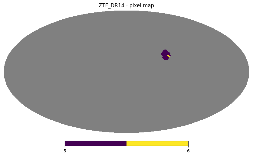
Throughout this notebook we will use the Catalog’s plot_pixels method to display the HEALPix of each resulting catalog as filters are applied.
[6]:
ztf_object.plot_pixels("ZTF_DR14 - pixel map")
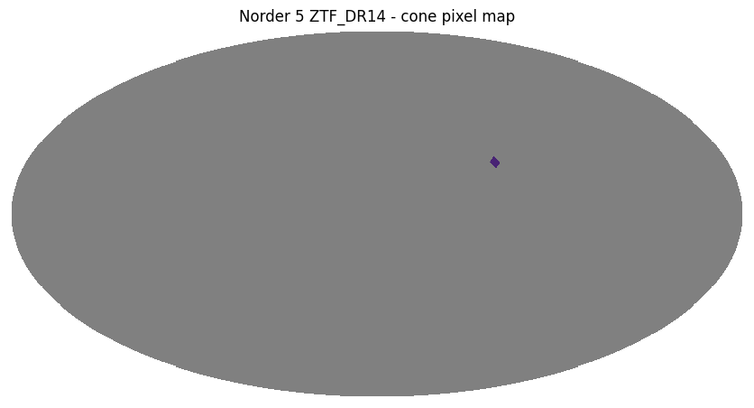
Cone search#
A cone search is defined by center (ra, dec), in degrees, and radius r, in arcseconds.
[7]:
ztf_object_cone = ztf_object.cone_search(ra=-60.3, dec=20.5, radius_arcsec=1 * 3600)
ztf_object_cone
[7]:
| ps1_objid | ra | dec | |
|---|---|---|---|
| npartitions=4 | |||
| 3645663898356416512 | int64[pyarrow] | double[pyarrow] | double[pyarrow] |
| 3646789798263259136 | ... | ... | ... |
| 3652419297797472256 | ... | ... | ... |
| 3653545197704314880 | ... | ... | ... |
| 18446744073709551615 | ... | ... | ... |
[8]:
ztf_object_cone.plot_pixels("ZTF_DR14 - cone pixel map")
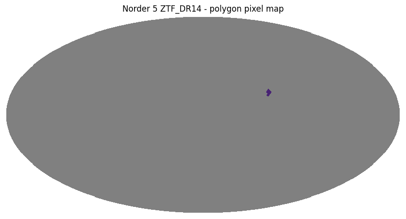
Polygon search#
A polygon search is defined by convex polygon with vertices [(ra1, dec1), (ra2, dec2)...], in degrees.
[9]:
vertices = [(-60.5, 15.1), (-62.5, 18.5), (-65.2, 15.3), (-64.2, 12.1)]
ztf_object_polygon = ztf_object.polygon_search(vertices)
ztf_object_polygon
[9]:
| ps1_objid | ra | dec | |
|---|---|---|---|
| npartitions=5 | |||
| 3614138700964823040 | int64[pyarrow] | double[pyarrow] | double[pyarrow] |
| 3638908498915360768 | ... | ... | ... |
| ... | ... | ... | ... |
| 3642286198635888640 | ... | ... | ... |
| 18446744073709551615 | ... | ... | ... |
[10]:
ztf_object_polygon.plot_pixels("ZTF_DR14 - polygon pixel map")
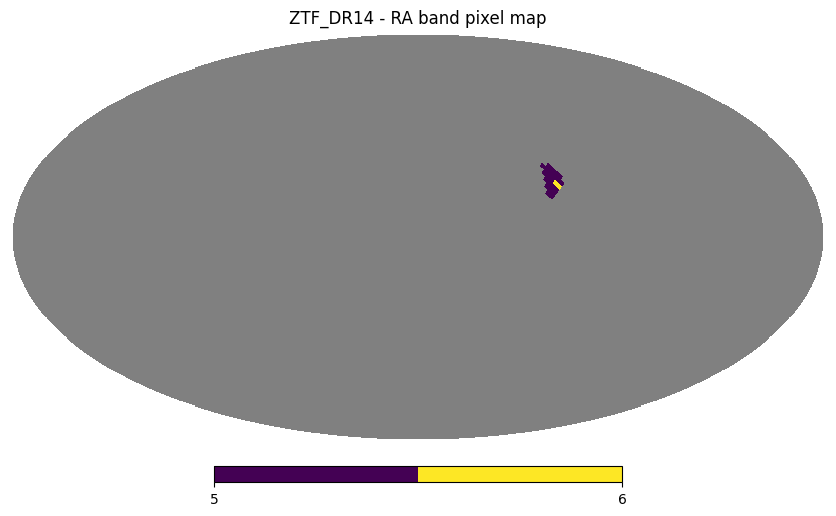
Box search#
A box search can be defined by:
Right ascension band
(ra1, ra2)Declination band
(dec1, dec2)Both right ascension and declination bands
[(ra1, ra2), (dec1, dec2)]
Right ascension band#
[11]:
ztf_object_box_ra = ztf_object.box(ra=[-65, -60])
ztf_object_box_ra
[11]:
| ps1_objid | ra | dec | |
|---|---|---|---|
| npartitions=30 | |||
| 3614138700964823040 | int64[pyarrow] | double[pyarrow] | double[pyarrow] |
| 3615264600871665664 | ... | ... | ... |
| ... | ... | ... | ... |
| 4053239664633446400 | ... | ... | ... |
| 18446744073709551615 | ... | ... | ... |
[12]:
ztf_object_box_ra.plot_pixels("ZTF_DR14 - RA band pixel map")
Declination band#
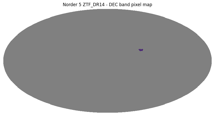
[13]:
ztf_object_box_dec = ztf_object.box(dec=[12, 15])
ztf_object_box_dec
[13]:
| ps1_objid | ra | dec | |
|---|---|---|---|
| npartitions=5 | |||
| 3613012801057980416 | int64[pyarrow] | double[pyarrow] | double[pyarrow] |
| 3614138700964823040 | ... | ... | ... |
| ... | ... | ... | ... |
| 3638908498915360768 | ... | ... | ... |
| 18446744073709551615 | ... | ... | ... |
[14]:
ztf_object_box_dec.plot_pixels("ZTF_DR14 - DEC band pixel map")
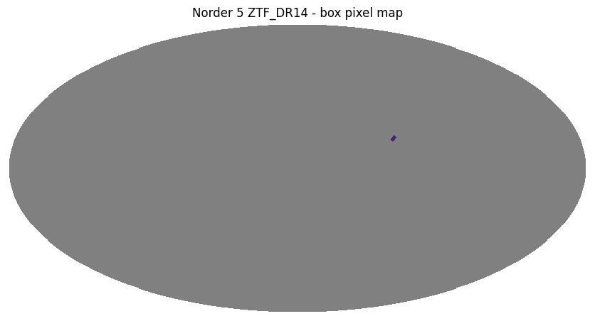
Right ascension and declination bands#
[15]:
ztf_object_box = ztf_object.box(ra=[-65, -60], dec=[12, 15])
ztf_object_box
[15]:
| ps1_objid | ra | dec | |
|---|---|---|---|
| npartitions=2 | |||
| 3614138700964823040 | int64[pyarrow] | double[pyarrow] | double[pyarrow] |
| 3638908498915360768 | ... | ... | ... |
| 18446744073709551615 | ... | ... | ... |
[16]:
ztf_object_box.plot_pixels("ZTF_DR14 - box pixel map")
We can stack a several number of filters, which are applied in sequence. For example, catalog.box().polygon_search() should result in a perfectly valid HiPSCat catalog containing the objects that match both filters.
Previewing part of the data#
Computing an entire catalog requires loading all of its resulting data into memory, which is expensive and may lead to out-of-memory issues.
Often our goal is to have a peek at a slice of data to make sure the workflow output is reasonable (e.g. to assess if some new created columns are present and their values have been properly processed). head() is a pandas-like method which allows us to preview part of the data for this purpose. It iterates over the existing catalog partitions, in sequence, and finds up to n number of rows.
Notice that this method implicitly calls compute().
[17]:
ztf_object_cone.head()
[17]:
| ps1_objid | ra | dec | |
|---|---|---|---|
| _hipscat_index | |||
| 3646116619639324672 | 131432999494754032 | 299.949481 | 19.527901 |
| 3646116620503351296 | 131432999482554346 | 299.948273 | 19.52819 |
| 3646116620964724736 | 131432999472704717 | 299.94726 | 19.528454 |
| 3646116621937803264 | 131432999480965958 | 299.948077 | 19.529494 |
| 3646116750698741760 | 131442999840264659 | 299.984096 | 19.536824 |
By default the first 5 rows of data will be shown but we can specify a higher number if we need.
[18]:
ztf_object_cone.head(n=10)
[18]:
| ps1_objid | ra | dec | |
|---|---|---|---|
| _hipscat_index | |||
| 3646116619639324672 | 131432999494754032 | 299.949481 | 19.527901 |
| 3646116620503351296 | 131432999482554346 | 299.948273 | 19.52819 |
| 3646116620964724736 | 131432999472704717 | 299.94726 | 19.528454 |
| 3646116621937803264 | 131432999480965958 | 299.948077 | 19.529494 |
| 3646116750698741760 | 131442999840264659 | 299.984096 | 19.536824 |
| 3646116752913334272 | 131442999792923350 | 299.979209 | 19.535608 |
| 3646116753051746304 | 131442999803743832 | 299.980368 | 19.536026 |
| 3646116753819303936 | 131442999770212613 | 299.977055 | 19.535172 |
| 3646116754284871680 | 131442999775374201 | 299.977557 | 19.536359 |
| 3646116755371196416 | 131442999790335818 | 299.97904 | 19.537692 |
Closing the Dask client#
[19]:
client.close()